In this article, we will explore more about Regression Algorithm. We will learn about Polynomial Regression in this blog.
Before starting the post you will need the following pre-requisites.
Pr-Requisites
- Python and its library. Matplotlib, Numpy, and Pandas are highly recommended and we are going to use these three libraries.
- Knowledge of Simple Linear Regression.
Check out my post on Simple Linear Regression to learn more about it.
Table of Contents
- What is Polynomial Linear Regression and Why to use this algorithm?
- Implementation in Python
What is Polynomial Linear Regression?
In Simple Linear Regression, we use a straight line with formula Y = MX + C.
It was used to best fit the line to our dataset.
But in some datasets, it is hard to fit a straight line. Therefore we use a polynomial function of a curve to fit all the data points.
Let’s consider the following data set.

To get the data set Click the link below so you can follow along.
https://www.kaggle.com/uciml/autompg-dataset
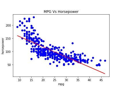
In this data set as you can see that the data points are in the curved area.
So it’s hard to fit the straight line to this dataset.
The formula of the polynomial linear regression is almost similar to that of Simple Linear Regression.
y = b0 + b1 x + b2 x2 +⋯ +bn xn
So let’s implement the algorithm in Python.
Implementation of the polynomial linear regression in Python
First, we will import all the libraries we need for this tutorial.
After that, we will get out the data set and data points.
import numpy as np
import pandas as pd
import matplotlib.pyplot as pltdata = pd.read_csv('Auto.csv')
X = np.array(data['mpg'].values).reshape((-1,1))
y = np.array(data['horsepower'].values).reshape((-1,1))
First of all, we will fit the linear regression model to our data set. So that we can compare it with our polynomial model.
# Fitting Linear Regression to the dataset
from sklearn.linear_model import LinearRegression
lin_reg = LinearRegression()
lin_reg.fit(X,y)
If you are not familiar with the simple linear regression I recommend you to first learn that and then continue this algorithm.
After that, we will fit our polynomial model. To do that we will import PolynomialFeatures from sklearn.
# Fitting Polynomial Regression to the dataset
from sklearn.preprocessing import PolynomialFeatures
After importing we will create an object of the polynomial feature and then fit our model.
poly_reg = PolynomialFeatures(degree = 3)
X_poly = poly_reg.fit_transform(X)lin_reg2 = LinearRegression()
lin_reg2.fit(X_poly,y)
Now we will visualize the simple linear regression algorithm first.
# Visualising the Linear Regression
plt.title("MPG Vs Horsepower")
plt.xlabel('mpg')
plt.ylabel('horsepower')
plt.scatter(X, y, color = "blue")
plt.plot(X,lin_reg.predict(X),color = "red")
plt.show()
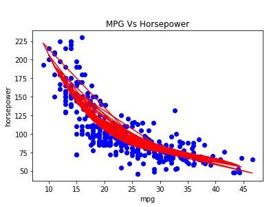
After that, we will visualize our algorithm.
# Visualising the Polynomial Regression
plt.title("MPG Vs Horsepower")
plt.xlabel('mpg')
plt.ylabel('horsepower')
plt.scatter(X, y, color = "blue")
plt.plot(X,lin_reg2.predict(poly_reg.fit_transform(X)),color = "red")
plt.show()
Conclusion
In conclusion, Polynomial Linear Regression is used with complex data sets in which we can not fit a straight line.
In the next post, we will learn about Decision Trees so Stay Tuned.
Resources
https://scikit-learn.org/stable/modules/preprocessing.html#generating-polynomial-features
